Using Gradient Descent for Life Optimization

the interesting part is how do we define the function?

Oct 10, 2021

A few days ago, a friend sent me an article in Chinese talking about philosophical interpretations of SGD (Stochastic Gradient Descent). The author raises an interesting viewpoint that “SGD can be used for life optimization”, which triggers me to think about the correlations between life and gradient descent algorithms in general. This newsletter may require some understanding of ML and math background. Since substack doesn’t support Latex integration, I need to use LaTex to type out the math expressions.

Recap

What is the gradient descent algorithm? In short, it is an iterative optimization algorithm for finding a minimum of a differentiable function. The intuition behind the method is calculus. Calculus says that a function f differentiable at a point w can be locally well approximated by a linear function, namely

This is analogous to drawing a tangent line to the graph of a univariate function ( when n = 1). It’s intuitively clear that the tangent line approximates the function well near the point of approximation, but not generally for faraway points.

In a linear function:

we just move in the direction -c, for a rate of decrease of \norm{c}_2. Similarly, for f(w), we move in the direction of -\nabla{f(w)}, and stop when once the improvement is too small to bother with. Gradient descent’s part of the contract is to only take a small step (as controlled by the parameter α below) so that the guiding linear approximation is approximately accurate.

In human language, to find the local minimum of a function using gradient descent, we take steps proportional to the negative of the gradient (moving away from the gradient) of the function at the current point. Under mild consumption, gradient descent converges to a local minimum. If f is convex - meaning all chords lie above its graph - then gradient descent converges to a global minimum.

Define the Life optimization problem

Okay, I believe we have all the basic knowledge about gradient descent. Now it’s time to relate it to our life, and use this beautiful algorithm to optimize it.

Imagine we have numerous data points in life in the form of:

For each dimension, we can view it as an aspect of effort in life. For example, nutrition, exercise, languages, time allocation, or sleeping habits. x means what we actually do in life, and y means the corresponding result. The goal is to find the perfect utilization in each of the dimensions just like tuning parameters of a model - how much strength do we need in each of the aspects.

To begin the training, it’s important to find the objective of life. In machine learning, the objective is usually to minimize a loss function, which can be logistic loss or squared error loss… In life, we want to reach some lifetime goals rhetorically like climbing a summit, to maximize our lives. It’s basically the same question with a matter of the sign, we find the minimum and flip the parabola, then it’ll be the maximum.

Then, the interesting part is how do we define the function? The function here is a symbolic interpretation of goals in life. Different people have different goals in life: the objective can be to maximize wealth, happiness, reputation, social impacts, or even appearance, as long as the goal is high enough so that the function is convex. But some may ask, what if I want multiple goals in life at the same time? What if people want both wealth and happiness? Actually, this is feasible too, we can just simply add those goals together. The sum of convex functions is also convex. In theory, by using gradient descent, we’ll eventually arrive at the destination after many iterations in time series.

Let’s give one simple example here. Alice is a high school student and her goal is to attend a good university. If Alice uses gradient descent as an optimization algorithm, the objective for her is to go to the most prestigious school possible, like Harvard or MIT. Her life events are data points we use to train the model, we record how she behaves in multiple dimensions and the corresponding results comparing to her objective. Is Alice focused in classes? Does Alice have enough sleep? Does she have regular exercise? How much time she spent practicing piano… And based on the allocation of Alice’s effort, the results are her SAT scores, her leadership in clubs or community, her extracurriculars, and her place in piano competition ... In the application, gradient computation means she examines her practices based on the corresponding results. The “descent” part is she makes micro-steps continuously and frequently to rationalize the adjuments. Freshmen year, Alice was sick for 1 month and missed all classes, the optimal solution for next quarter is to exercise more and eat nutritious food to avoid illnesses. Sophomore year, Alice had a high GPA but failed the election of the president in her chess club. Her choices would be practicing public speaking skills and compassion for peers. And each year, she would make adjustments like this to work for her dream college.

Become a Better Player

In this article mentioned above, the author discussed the philosophies of the algorithm. I agree with most of them and have my own interpretations of using gradient descent as a life optimization too.

Choosing the proper learning rate

Choosing a proper learning rate can be difficult. A learning rate that is too small leads to painfully slow convergence, while a learning rate that is too large can hinder convergence which causes the loss function to fluctuate around the minimum or even to diverge.

Smart people always find a good learning pace to grow. They will push themselves forward hard enough, but not too aggressively to burn out.

Stochastic approach

Source: http://www.its.caltech.edu/~nazizanr/papers/SMD.html

Stochastic gradient descent comes in as a trade-off between the number of iterations and the computation required per iteration. Ideally, you want as much data as possible since more data allows you to learn richer and more accurate models (excludes overfitting). However, it can be problematic to spend too much time computing every single iteration of gradient descent. Instead of asking all data points for their votes, we only ask for the opinion of a single randomly chosen data point — the dictator for this iteration.

The first takeaway from the stochastic approach is, we don’t need a large set of data points in life for optimization. You’ll be distracted and running much slower if you focus on every granular detail of life events. Another implementation note of SGD is that a poor choice of a data point can lead you in the complete opposite direction. So the second takeaway is, even though you need some randomness in your exploration of life, don’t go for an extreme case.

The path is unique

https://en.wikipedia.org/wiki/Stochastic_gradient_descent

Following up with SGD, or even using “mini-batches” for data selections, we need to admit that there’re always some uncertainties in the process even using the right approach. Setting up the same objective and run the algorithm many times, you’ll never get the same path. It is meaningless to look at each gradient in every epoch and compare its effectiveness.

In the same game in life, we pick up different points on the different stages of the journey. The data point is special to every one of us depended on various internal or external factors. We don’t need to compare our own path with anyone else. Just enjoy the ride.

Never give up

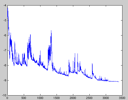
With any starting point of the objective function, we’ll always converge at the local/global minimum in time. If you haven’t, it only means that you haven’t tried enough numbers of iteration.

Nothing in this world can take the place of persistence. If you have a dream, hold on to it. If you believe in what you are doing, never give it up. The path might fluctuate a little bit but don’t be discouraged, anything takes time. It is okay that you are burned out and are lost in the track. Just pick up where you fell and start tuning your life from there. If the algorithm is guaranteed to converge to within some range of the optimal value, we’d better hold up to it as long as we can.

Limitations of the Algorithm

Not a convex function altogether

The sum of convex functions is also convex but what if the two functions cancel each other out and causing a negative-sum? It’s not true in the math world, but it happens a lot in real life. Imagine having a good career as a convex function, and taking good care of families also as a convex function. Independently, they are excellent goals, but sometimes there’s no way to maintain both. This is a bad example, but imagine your kid is terribly injured and needs to be taken care of at the hospital while you need to attend a really important company-wise meeting the same day. If you choose to stay in the hospital to take care of your kid, you will lose the credits you deserved and the investment you worked years for. If you go to the meeting, you will be guilty of your family and may not perform well in the meeting. Moreover, the relationship between you and your kid may grow apart. There will be regressed consequences no matter what you choose, 1 + 1 can be less than 2, or even less than 0.

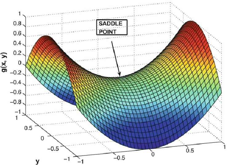
Trapped in Saddle point

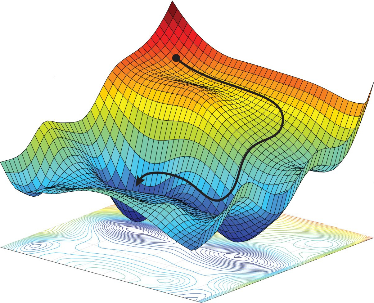
Figure no. 5: Example of saddle point in error surface caused by too... | Download Scientific Diagram

The key challenge of minimizing highly non-convex functions common for neural networks is avoiding getting trapped in their numerous suboptimal local minima. Moreover, the difficulty arises in fact not from local minima but from saddle points, points where one dimension slopes up and another slopes down. These saddle points are usually surrounded by a plateau of the same error, which makes it notoriously hard for SGD to escape, as the gradient is close to zero in all dimensions.

There are saddle points in life too. You think you have reached the global minimum and you stop the optimization, but you are just in the local minimum. It’s hard to get out there since you are in your comfort zone for too long and lose the ability to compute gradients.

The function is not differentiable

Sometimes, the function is not differentiable. Take the graph above as an example. At x1, the convex function f is differentiable, and g1 (which is the derivative of f at x1) is the unique subgradient at x1. At the point x2, f is not differentiable. At this point, f has many subgradients: two subgradients, g2 and g3, are shown.

There are many subgradient methods such as the projected subgradient method that solve the constrained convex optimization problem. The subgradient method uses step lengths that are fixed ahead of time, instead of an exact or approximate line search as in the gradient method. However, it is not a descent method (the function value can and often does increase). It needs to be used with primal or dual decomposition techniques, which can be more complicated.

Limited computational power and a finite number of iterations

Different people have different hardware for various reasons. Some compute gradients faster while others have less reliable machines that cause longer computational time per iteration. One solution I can think of is to reduce the number of dimensions in the function - this means we need to focus on the more essential aspects of life during the training process.

Our lifetime is limited as well. Some live longer, and others live shorter. It’s likely that we run out of time before the life function converges.

Conclusion

After all, using SGD as a life optimization method is just an interesting analogy. Some points in this article are arguably incomplete or incorrect. Hopefully, this brings more thinkings and discussions. There are still more blanks to fill at the theoretical level.